The options book manager provides the modeling and experimentation features sophisticated enough to handle the most demanding option books. It offers a single place to analyze how potential adjustments impact the expectations for a given underlying, as well as the overall portfolio.
Watch our YouTube series on the book manager. We will also call out specific videos from this series below.
Launching the book manager
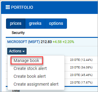
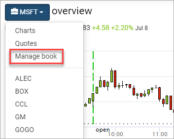
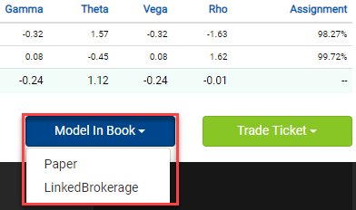
There are multiple ways to get to the book manager for a given stock. The easiest is to select Manage book from the Actions dropdown in your portfolio. Alternatively, you can navigate to a book from the symbol dropdown in the breadcrumb from a stock’s overview.
You can also send a trade from the trade analyzer or option chart to the book manager to see how it impacts your current holdings.
Understanding books
Quantcha uses the term book to refer to the entire set of equity and option holdings for a given underlying in the current portfolio. The book manager keeps track of two different books for the current underlying: the current book and the pending book.
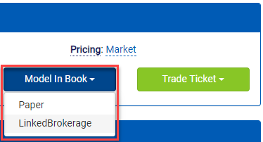
The current book reflects the actual holdings of the selected portfolio. If you are using the built-in paper portfolio, then these are positions you have either imported from a brokerage export or have entered manually. If you are using a linked brokerage account, then these are the positions reported from the brokerage API. The current book is generally detailed using the color blue.
The pending book represents the potential state of the book. As you make changes in the book manager (or send in trades from other tools in the suite), the pending book is updated to reflect those changes. The default state of the pending book is identical to the current book until you start making changes. Once changes are made, the pending book uses the color yellow.
A book scenario
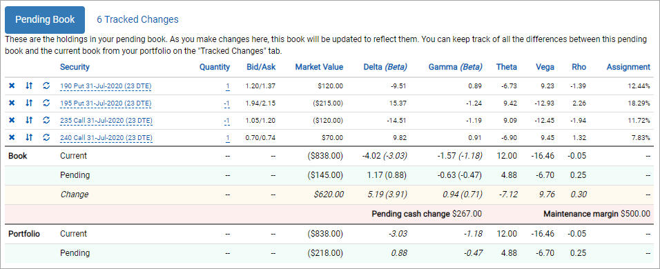
The screenshot below represents the scenario where the investor currently holds an iron condor position. They are experimenting the potential of rolling into a different iron condor trade. The positions shown here only represent the pending book as the current positions are generally irrelevant when adjusting a strategy. We will continue to use this scenario throughout this walkthrough.
Tracking changes
As changes are made to the pending book, the net changes required to move from the current state to the pending state are tracked in the Tracked Changes tab. These changes already account for any redundant trades, such as by cancelling out any purchases and sales of the same option. As a result, an investor can feel comfortable adding, removing, and adjusting positions to model the ideal results. The book manager will cut through everything to produce the most efficient trade adjustment plan.
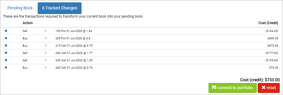
Revisiting the scenario outlined above, observe the tab that indicates that there are 6 Tracked Changes. This is because the new iron condor position being rolled into shares the same leg as the current trade. As a result, the book manager recognizes that there is no need to change that holding to meet the target state. Selecting that tab will outline the adjustment trade plan.
This was a relatively simple scenario to model because it was just closing part of one trade and opening part of another. However, things could get much more complex if trading volatility using various options selected from an option chart or multiple trades from the options search or a global screener.
If working with the paper portfolio, you will need to manually place these trades with your brokerage. Once completed, you can select commit to portfolio to automatically apply these changes to the Quantcha portfolio. If you’re working from a linked brokerage account, you will instead see a trade button that will lead you to a populated trade ticket. However, you may need to place multiple orders to execute a plan like this if you brokerage doesn’t support six-legged trades.
Watch our video on book management.
Adjusting a book
There are three ways to change positions in the pending book. One way is to send trades to the book manager from other tools in the suite, as shown earlier. Let’s discuss the other two options.
Adjusting positions in line
Each position in a pending book includes shortcut buttons to close or invert the position. You can also adjust the quantities of existing positions by selecting the position to reveal an editable quantity field.
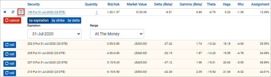
There is also a roll button that simplifies the process of swapping one option for another of the same type and quantity. Each potential roll displays the cost (or credit) for that position change, as well as its Greeks.
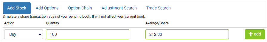
Adding positions
Stock and option positions may be manually added to the pending book using the options to add stock or options from the bottom of the view. If you know the specific options you’re looking for, you can use the Add Options tab. Otherwise you can scan the Option Chain.
Searching for adjustments
The book manager also offer an automated adjustment search. This feature allows you to specify the target goals for your book, such as a delta range, as well as option properties, such as an expiration range or budget.
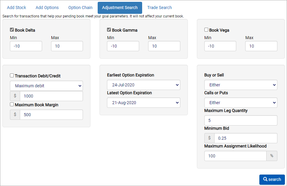
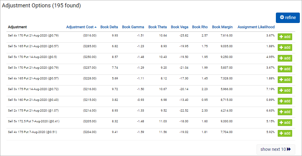
The search then digs out the best potential single-leg adjustments you can make to meet your target. Click add to apply that leg to your pending book.
Modeling returns
The book manager includes a set of modeling visualizations to help you understand how pending changes impact the expected returns for your book.
Profit & loss projection
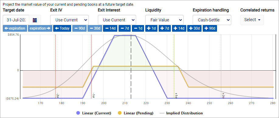
The profit & loss projection is a configurable chart that models the expected returns for both the current and pending books. Note that this models returns relative the current market value of any existing holdings you already have.
Target date
Specifies the date the projections are modeled for. By default, this is the first expiration used in the current or pending books. There are shortcut buttons below to make it easier to jump to different expirations, as well as by absolute days.
Exit implied volatility (IV)
Specifies the implied volatility strategy to use for valuing options that are still open on the target date. There are several options:
- Use Current is the default option and uses the current IV of the options to price them on the target date.
- Infer From Surface attempts to infer the future implied volatility based on the current surface. For example, if a given call will be 15% in the money and 17 days from expiration on the target date, it will be priced using the interpolated implied volatility for those parameters on the current volatility surface.
- Use Custom IV allows the user to specify an exact IV to use for all option modeling on the target date.
Exit interest
Specifies the risk-free interest rate to use for valuing options that are still open on the target date. There are two options:
- Use Current is the default option and uses the current risk-free rate to price options on the target date.
- Use Custom Rate allows the user to specify the rate to use for all option modeling on the target date.
Liquidity
Specifies the liquidity strategy to use for valuing the prices at which options will need to be closed at when they reach expiration. There are two options:
- Fair Value is the default option and uses the intrinsic value of the option, assuming there will be no liquidity cost (bid and ask are modeled at intrinsic value).
- Infer Liquidity attempts to infer the future liquidity costs based on the current surface. For example, if a given call will be 15% in the money and 17 days from expiration on the target date, the size of its bid/ask spread will be priced using the interpolated liquidity for those parameters on the current liquidity surface.
Watch our video on book valuation.
Expiration handling
Specifies the expiration handling strategy to use for closing in-the-money option positions when they reach expiration. There are several options:
- Cash-Settle is the default option and buys or sells the positions to close at expiration.
- Always Exercise assumes all options will be exercised or allowed to be assigned if they are in the money at expiration.
- Exercise If Covered exercises or allows the assignment of options that are in the money if a sufficient amount of the underlying is held at the time.
Watch our video on expiration handling.
Correlated returns
Sometimes a trade strategy will involve equity or option positions from multiple underlying securities. The correlated returns feature enables you to modeling those holdings in with the current book and chart it relative to the current underlying’s price. This sophisticated modeling technique uses correlations between all selected underlyings, along with their implied volatilities, to project feasible price paths for all securities involved.
For example, let’s say you hold SPY calls and hedge them with SPXS calls (leveraged inverse of SPY). To more effectively model the expected adjustments to your SPY book, you would want to include your SPXS book as part of the modeling process. Note that correlated returns don’t require the underlyings to have an absolute relative beta of 1. You can run this technique with any combination of optionable stocks, such as two tech stocks you’re pair trading. However, the less correlation the underlyings have, the more unpredictable their relative performance will be.
Price path modeling
A price path is the progression of prices an underlying may follow between today and the target date. In general, the only prices of interest between the two dates are those where options are set to expire. The book manager offers two price path modeling strategies: linear progression and Monte Carlo.
Watch our price path modeling video.
The linear progression price path modeling strategy models the expected price movement between two dates using the implied volatility for that term. This is the ideal option for scenarios where the target date occurs before or at the first option expiration. When prices at one or more expiration dates between today and the target date must be projected, linear progression attempts a trending model that distributes each path’s price movement along the terminal path. As a result, this strategy is notably less reliable when used beyond the first option expiration date.
Watch our linear progression pricing video.
The Monte Carlo path modeling strategy uses a large quantity of simulations that represent appropriately scaled movements between any two dates. These movements are based on probabilities extracted from the implied volatility for those two points in time. Linear progression should be preferred when working with dates up until the first expiration, and Monte Carlo used for dates beyond.
Watch our Monte Carlo pricing video.
Revisiting the scenario
The screenshot above illustrates the different return profiles for the current and pending books in our scenario. The blue line indicates that the current holdings offer a greater potential return, but the pending book offers a wider strike range of profit. Since all options expire on the target date, the lines offer crisp corners and edges.
Let’s see what happens if we pull in the target date by one week.
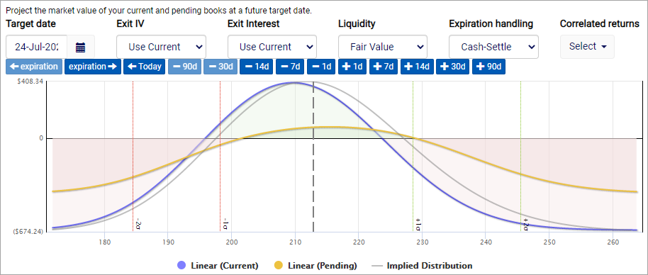
Observe that both returns are now expressed as fluid curves, which represents the varied returns that are projected for each terminal price in the range. Also notice that the implied distribution, shown in gray, represents a smaller total range due to the shorter term.
Now let’s see what kind of liquidity penalty we should expect if we need to close this trade on that day by opting to infer liquidity from the surface.
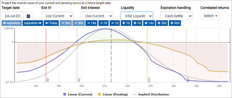
As you can see, the price expectations drop quite a bit, especially if the underlying makes a big move. This doesn’t mean you wouldn’t be able to get a better fill, but it gives you an idea of what to expect based on current market conditions.
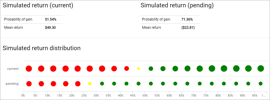
Simulated returns
In addition to modeling the profit & loss expectations for the term, the book manager also produces a simulated return analysis. This analysis uses a Monte Carlo modeling of the current and pending books to produce a large number of feasible outcomes.
The simulated returns indicate the percentage of simulations produced a profit, as well as what the mean return was. Investors will often find that adjustments result in a tradeoff between the probability of profit and expected mean return.
The simulated return distribution force ranks the returns into 20 buckets for a side-by-side return visualization. Each circle represents the relative size of that bucket’s returns in order to appreciate the distribution of returns. For example, the majority of simulations produced roughly the same profit for the pending book, whereas the profit potential for the current book were more concentrated among a smaller number of simulations.