
Exercise: Projecting future book value
One of the most important features every investor needs is the ability to project the market value of their investment in the future. With options, there are a variety of pricing factors that impact the value of each position, including the price of the underlying, days until expiration, interest rates, and implied volatility. The Profit & Loss Projection (P&L) section provides a flexible and intuitive way to model both your current and pending books.
Before continuing, it’s recommended that you watch Portfolio and book management video series. This series explains many of the concepts in this topic in depth.
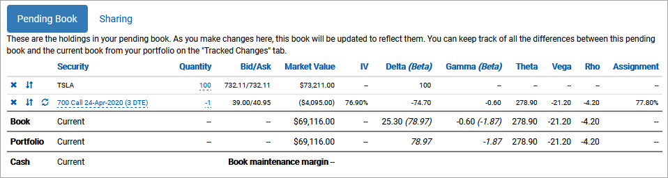
When you imported the exercise portfolio, it included a covered call strategy for TSLA. This included two legs: 100 shares and a short call struck at 700 for April 24 (2 DTE). This book will be used throughout this topic.
Scroll down to review the pending book that lists these positions. Return to the P&L at the top when done.
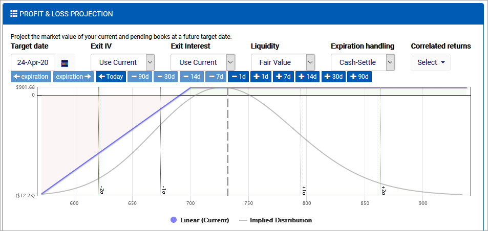
The P&L lays out the projected returns (relative to current value) by plotting the change in book value in dollars on the vertical axis. The horizontal axis uses a 3-vol (standard deviation) move that represents the underlying closing price on the selected date.
Book manager configuration
There are six configurable parameters that can be used to define how the book should be priced in the future.
- Target date is the date to project for. The prices on the horizontal axis are closing prices on that day. Since a book may contain options with different expirations, there is no option for “days until expiration” (DTE).
- Exit IV defines the strategy for selecting an IV to use for evaluating active (DTE > 0) options on the target date.
- Use Current applies the current IV of the option when evaluating its price on the target date.
- Infer From Surface uses an interpolation model that determines the likely IV for an option with its moneyness and DTE based on the current volatility surface.
- Use Custom IV allows you to specify a specific IV to use for all target date calculations.
- Exit Interest defines the strategy for selecting an interest rate to evaluate active options on the target date.
- Use Current uses current interest rates.
- Use Custom Rate allows you to specify a rate to use.
- Liquidity defines the strategy to use for calculating the liquidity cost to close active options. For example, an option with a fair price of 1.00 may have a bid/ask spread of 0.95/1.05.
- Fair Value uses the expected value of the option as-is based on the specified pricing parameters. In the example above, this would value the option at 1.00.
- Infer Liquidity uses an interpolation model that determines the likely option liquidity for an option with its moneyness and DTE based on the current liquidity surface. In the example above, long options would be marked at 0.95 to close, whereas short options would be marked at 1.05 to close.
- Expiration handling defines the strategy to use for handling options that expire on or before the target date.
- Cash-Settle always buys or sells the option to close, regardless of any position in the underlying stock.
- Always Exercise exercises or allows assignment of in-the-money (ITM) options at expiration, which may result in a position in the underlying. When that happens, the underlying position is tracked through to the target date like any other position.
- Exercise If Covered exercises or allows assignment on ITM options at expiration if there are offsetting ITM options with the same expiration or an underlying position to support it. Otherwise positions are cash-settled.
- Correlated returns specifies which other books should be included in the P&L. This modeling uses a sophisticated technique to project relative price movements between two or more books based on their historical correlation. This is especially useful when evaluating highly [positively or negatively] correlated underlyings, such as when hedging one ETF with a position in its inverse ETF.
Note how the P&L is a well-defined line with one inflection point. That’s because the book manager defaults to the first expiration when opening a book. In this case, the covered call position expires in two days, on April 24.
Drag your mouse along the P&L curve to see how the change tops out at $884 and stays flat above the option strike price of $700.
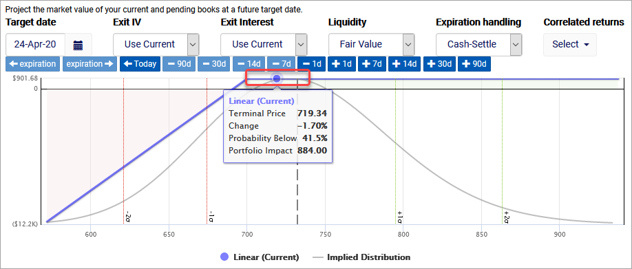
Hovering over the P&L line provides some insight as to the return at that price. It includes the the terminal price of the underlying, the change that price represents relative to the current underlying price, the probability the underlying will close below that price, and the total impact that price would have on your portfolio based on the configured parameters.
Modeling dates beyond the first expiration
However, you’re not limited to working with expiration dates. For example, what if you’ve decided to hold this position through this week’s expiration and want to evaluate the expected P&L at the end of next week?
Click the +7 button to change the Target date to May 1. This is a week after the short option held is set to expire.
Hover the mouse along the P&L to examine the projected change in value.
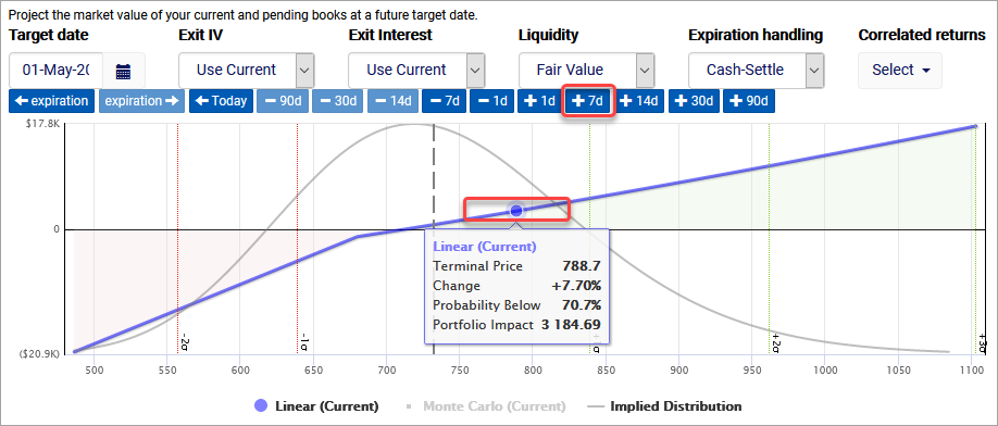
Notice how the P&L doesn’t stay flat above the $700 strike anymore. This is because the book manager is modeling through the next expiration on April 24. If the option is ITM, it’s going to buy it to close, otherwise it will let it expire. Then it will model the following week, which is just 100 shares of stock. Part of the reason this chart is so smooth is because of the default price path modeling strategy: linear progression pricing.
The book manager employs two price path modeling strategies:
- Linear progression pricing models the price movement of the underlying based on relative volatility movements. In other words, it models 1-vol movements between different milestones in a book’s future in order to form a smooth price path that represents expectations if the stock marched toward a terminal price in a consistent way. This is ideal for modeling prices up through the first expiration, but loses reliability as additional expirations are included.
- Monte Carlo pricing uses statistically feasible random movements to create a sample set of price paths for evaluation. Since it’s randomized, this modeling method doesn’t produce exhaustive results, but does provide more realistic results than linear progression across multiple expirations.
Select Monte Carlo (Current) to add a chart series for Monte Carlo pricing.
Hover your mouse over one of the sample points that indicates a loss above the current price. Since these points are generated randomly, they will not exactly match the screenshot below.
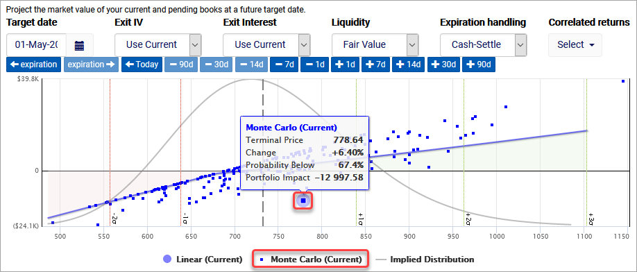
Notice how the Monte Carlo pricing has a lot of overlap with the linear progression pricing for lower prices, but then diverges quite a bit for higher prices. This is because Monte Carlo supports the scenario where the stock rises (or falls) prior to the first expiration, but then moves in the opposite direction in the second week. If you see cases where there is a market value loss despite the underlying rising, it’s because the underlying rose enough to make closing the call expensive, but then dropped afterwards, resulting in the stock position losing some value and netting a loss relative to today’s value.
The main reason the Monte Carlo points show so much divergence is because the short call is being cash settled at expiration, per the handling strategy. However, what would happen if we allowed the option to be assigned at expiration, calling away the shares?
From the Expiration handling dropdown, select Exercise If Covered.
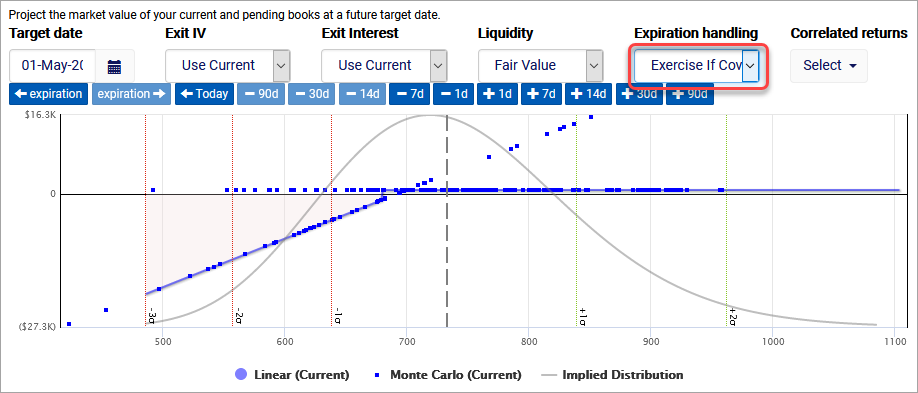
Now that the book manager has been instructed to allow assignment if covered, the Monte Carlo chart shows more uniformity. That’s because there are two different scenarios represented by their own lines made up of many Monte Carlo simulations.
- The horizontal line represents all the scenarios where the option was assigned and the stock was called away. In those cases, the trade closed on April 24 for full value because the assignment resulted in a flat (empty) book. It doesn’t matter where the stock ended up closing the week after because there was no position after assignment.
- The diagonal line represents all the scenarios where the stock dropped below the strike price, so the call expired and the shares were not called away. However, the stock then moved the next week, resulting in different outcomes based on the stock’s final price.
Modeling dates before expiration
There is often a need to model the value of a book containing options which have not yet reached expiration. In those cases, options are priced using the current configuration. Let’s see how that impact the current covered call projection.
Select the Today shortcut to change the Target date to “today”, which is April 22. The short leg expires two days later.
Locate the spot on the P&L around the terminal price of $740. Note the Portfolio Impact, which should be around $280. It doesn’t need to match exactly.
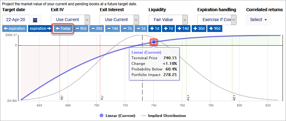
The first thing you may notice is that the Monte Carlo pricing has disappeared. That’s because linear pricing is ideal for modeling book value up until the first expiration. Since Monte Carlo doesn’t add any value, it’s removed from those terms.
Next, notice how the P&L is now a relatively smooth curve that reflects the change in value of this strategy a few days prior to expiration. Since the stock is currently trading around $732, we would expect 100 shares to be worth $800 more if it rose to $740. However, the P&L indicates that the book would only be worth around $280 more, which is because the short call is projected to be worth $520 more than it is now ($800 – $280).
However, that pricing is based on the fair value of the option. In the event that you were going to close the position, you would likely need to trade closer to the asking price for that option. This slippage is also known as the cost of liquidity. Fortunately, the book manager can account for that if you need a more precise projection of book value.
From the Liquidity dropdown, select Infer Liquidity.
Locate the spot on the P&L around the terminal price of $740. Note the Portfolio Impact, which should be lower than before to account for the liquidity hit.
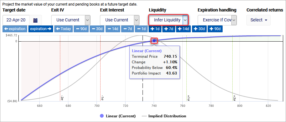
In this case, the liquidity cost of closing the short leg would be substantial and close to $2/share. This seems reasonable since the 700 call would be $40 ITM if the underlying moved up to $740. At the moment, the stock is trading at $732 and the 690 call (closest to $40 ITM) has a spread of 41.35/47.00. Of course, you’d possibly be able to improve on that by offering a price in the middle, but there’s no guarantee, so the book manager uses the market pricing.
Simulating returns
In addition to the P&L, the book manager provides two other return estimates based on the return simulations. The top set of Simulated return numbers aggregates the returns from all the price paths modeled to build the P&L and provides a probability of gain and a mean expected return.
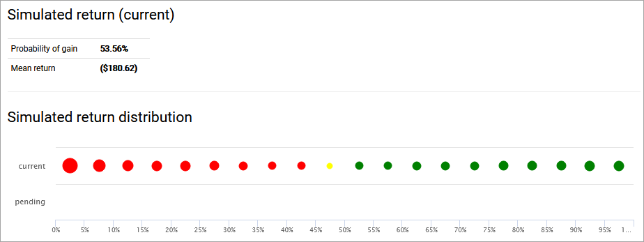
The bottom Simulated return distribution chart is a return distribution that groups simulated returns by magnitude so that you can understand the relative size of risk/reward across the distribution. It stack ranks each simulated return and displays each 5% group as a size relative to its total gain (green) or loss (red). The yellow dot represents the crossover point that contains some gains and some losses.